Tidy data 🧹

# Tidy data <br> 🧹

---

layout: true
  
<div class="my-footer">
<span>
<a href="https://rstd.io/bootcamper" target="_blank">rstd.io/bootcamper</a>
</span>
</div>

---

.your-turn[
Split into breakout groups and review a few questions from the "homework". If 
you did not have a chance to do the homework, that's fine. Use the sidebar to 
navigate to a topic that you were confused about and work on a few questions 
together. Take notes on topics you want to discuss/ask questions about when we 
come back to the big group.
]

---

# Tidy data

---

## Tidy data

>Happy families are all alike; every unhappy family is unhappy in its own way. 
>
>Leo Tolstoy

- Each variable forms a column.
- Each observation forms a row.
- Each type of observational unit forms a table.
]
--
.pull-right[
**Characteristics of untidy data:**

!@#$%^&*()
]

---

.footnote[
Source: [Army Air Forces Statistical Digest, WW II](https://www.ibiblio.org/hyperwar/AAF/StatDigest/aafsd-3.html)
]

---

<br>

.footnote[
Source: [Gapminder, Estimated HIV prevalence among 15-49 year olds](https://www.gapminder.org/data)
]

---

<br>

.footnote[
Source: [US Census Fact Finder, General Economic Characteristics, ACS 2017](https://factfinder.census.gov/faces/tableservices/jsf/pages/productview.xhtml?pid=ACS_17_5YR_DP03&src=pt)
]

---

## Summary tables

```
## # A tibble: 87 x 3
##   name           height  mass
##   <chr>           <int> <dbl>
## 1 Luke Skywalker    172    77
## 2 C-3PO             167    75
## 3 R2-D2              96    32
## 4 Darth Vader       202   136
## 5 Leia Organa       150    49
## 6 Owen Lars         178   120
## # … with 81 more rows
```
]
.pull-right[

```
## # A tibble: 3 x 2
##   gender    avg_height
## * <chr>          <dbl>
## 1 feminine        165.
## 2 masculine       177.
## 3 <NA>            181.
```
]
]

---

## Displaying data

```r
starwars %>%
  select(name, height, mass)
```

## Summarizing data

```r
starwars %>%
  group_by(gender) %>%
  summarize(
    avg_height = mean(height, na.rm = TRUE) %>% round(2)
  )
```

---

## A grammar of data tidying

.pull-left[
<img src="img/tidyr-part-of-tidyverse.png" width="70%" style="display: block; margin: auto;" />
]
.pull-right[
The goal of tidyr is to help you create tidy data
]

---

# Instructional staff employment trends

---

The American Association of 
University Professors (AAUP) is a nonprofit membership association of faculty 
and other academic professionals. 
[This report](https://www.aaup.org/sites/default/files/files/AAUP_Report_InstrStaff-75-11_apr2013.pdf) 
by the AAUP shows trends in instructional staff employees between 1975 
and 2011, and contains an image very similar to the one given below.

---

## Data

Each row in this dataset represents a faculty type, and the columns are the 
years for which we have data. The values are percentage of hires of that type 
of faculty for each year.

```r
staff <- read_csv("data/instructional-staff.csv")
staff
```

```
## # A tibble: 5 x 12
##   faculty_type          `1975` `1989` `1993` `1995` `1999` `2001` `2003` `2005` `2007` `2009` `2011`
##   <chr>                  <dbl>  <dbl>  <dbl>  <dbl>  <dbl>  <dbl>  <dbl>  <dbl>  <dbl>  <dbl>  <dbl>
## 1 Full-Time Tenured Fa…   29     27.6   25     24.8   21.8   20.3   19.3   17.8   17.2   16.8   16.7
## 2 Full-Time Tenure-Tra…   16.1   11.4   10.2    9.6    8.9    9.2    8.8    8.2    8      7.6    7.4
## 3 Full-Time Non-Tenure…   10.3   14.1   13.6   13.6   15.2   15.5   15     14.8   14.9   15.1   15.4
## 4 Part-Time Faculty       24     30.4   33.1   33.2   35.5   36     37     39.3   40.5   41.1   41.3
## 5 Graduate Student Emp…   20.5   16.5   18.1   18.8   18.7   19     20     19.9   19.5   19.4   19.3
```

---

## Recreate the visualization

In order to recreate this visualization we need to first reshape the data to have 
one variable for faculty type and one variable for year. In other words, 
we will convert the data from the long format to wide format.

But before we do so...

.discussion[
If the long data will have a row for each year/faculty type combination, 
and there are 5 faculty types and 11 years of data, how many rows will the data have?
]

---

---

## `pivot_*()` functions

![](img/tidyr-longer-wider.gif)

---

## `pivot_longer()`

```r
pivot_longer(data, cols, names_to = "name", values_to = "value")
```

- The first argument is `data` as usual.
--

- The second argument, `cols`, is where you specify which columns to pivot 
into longer format -- in this case all columns except for the `faculty_type` 
--

- The third argument, `names_to`, is a string specifying the name of the column to create from the data stored in the column names of data -- in this case `year`
--

- The fourth argument, `values_to`, is a string specifying the name of the column to create from the data stored in cell values, in this case `percentage`

---

## Pivot staff data

```r
staff %>%
  pivot_longer(
    cols = -faculty_type, 
    names_to = "year", 
    values_to = "percentage"
    )
```

```
## # A tibble: 55 x 3
##   faculty_type              year  percentage
##   <chr>                     <chr>      <dbl>
## 1 Full-Time Tenured Faculty 1975        29  
## 2 Full-Time Tenured Faculty 1989        27.6
## 3 Full-Time Tenured Faculty 1993        25  
## 4 Full-Time Tenured Faculty 1995        24.8
## 5 Full-Time Tenured Faculty 1999        21.8
## 6 Full-Time Tenured Faculty 2001        20.3
## # … with 49 more rows
```

---

## Pivot staff data, and save result

```r
staff_long <- staff %>%
  pivot_longer(
    cols = -faculty_type, 
    names_to = "year", 
    values_to = "percentage"
    )

staff_long
```

---

```r
staff_long %>%
  ggplot(aes(x = percentage, y = year, color = faculty_type)) +
  geom_col(position = "dodge")
```

![](05-tidy-data_files/figure-html/unnamed-chunk-13-1.png)

---

```r
staff_long %>%
  ggplot(aes(x = percentage, y = year, fill = faculty_type)) +
  geom_col(position = "dodge")
```

![](05-tidy-data_files/figure-html/unnamed-chunk-14-1.png)

---

## Some improvement...

```r
staff_long %>%
  ggplot(aes(x = percentage, y = year, fill = faculty_type)) +
  geom_col()
```

![](05-tidy-data_files/figure-html/unnamed-chunk-15-1.png)

---

## More improvement

```r
staff_long %>%
  ggplot(aes(x = year, y = percentage, group = faculty_type, color = faculty_type)) +
  geom_line()
```

![](05-tidy-data_files/figure-html/unnamed-chunk-16-1.png)

---

.your-turn[
- Go to RStudio Cloud and start the second assignment: `05 - Tidy Data`
- Open the first R Markdown file: `instructional-staff.Rmd`
- Knit the document, and work on the exercises
]

.footnote[
RStudio Cloud workspace for this bootcamp  
is at  [rstd.io/bootcamper-cloud](https://rstd.io/bootcamper-cloud).
]

---

![](05-tidy-data_files/figure-html/unnamed-chunk-18-1.png)

---

## Make year numeric again!

```r
staff_long <- staff_long %>%
  mutate(year = as.numeric(year))

staff_long %>%
  ggplot(aes(x = year, y = percentage, group = faculty_type, color = faculty_type)) +
  geom_line()
```

![](05-tidy-data_files/figure-html/unnamed-chunk-19-1.png)

---

![](05-tidy-data_files/figure-html/unnamed-chunk-20-1.png)

---

```r
staff_long %>%
* mutate(part_time = if_else(faculty_type == "Part-Time Faculty",
*                            "Part-Time Faculty",
*                            "Other Faculty")) %>%
  ggplot(aes(x = year, y = percentage/100, 
             group = faculty_type, 
             color = part_time)) + 
  geom_line() +
  scale_color_manual(values = c("gray", "red")) + 
  theme_minimal() + 
  labs(
    title = "Instructional staff employment trends",
    x = "Year",
    y = "Proportion",
    color = ""
  ) +
  theme(legend.position = "bottom")
```

---

```r
staff_long %>%
  mutate(part_time = if_else(faculty_type == "Part-Time Faculty", 
                             "Part-Time Faculty", 
                             "Other Faculty")) %>% 
  ggplot(aes(x = year, y = percentage/100, 
*            group = faculty_type,
*            color = part_time)) +
  geom_line() +
* scale_color_manual(values = c("gray", "red")) +
* theme_minimal() +
  labs(
    title = "Instructional staff employment trends",
    x = "Year",
    y = "Proportion",
    color = ""
  ) +
  theme(legend.position = "bottom")
```

---

![](05-tidy-data_files/figure-html/unnamed-chunk-23-1.png)

---

```r
*library(scales)
staff_long %>%
  mutate(part_time = 
           if_else(faculty_type == "Part-Time Faculty", 
                   "Part-Time Faculty", "Other Faculty")) %>% 
  ggplot(aes(x = year, y = percentage/100, group = faculty_type, 
             color = part_time)) +
  geom_line() +
  scale_color_manual(values = c("gray", "red")) +
* scale_y_continuous(labels = percent) +
  theme_minimal() +
  labs(
    title = "Instructional staff employment trends",
    x = "Year",
*   y = "Percentage",
    color = ""
  ) +
  theme(legend.position = "bottom")
```

---

![](05-tidy-data_files/figure-html/unnamed-chunk-25-1.png)

---

![](05-tidy-data_files/figure-html/unnamed-chunk-26-1.png)

---

```r
library(scales)
staff_long %>%
  mutate(part_time = 
           if_else(faculty_type == "Part-Time Faculty", 
                   "Part-Time Faculty", "Other Faculty")) %>% 
  ggplot(aes(x = year, y = percentage/100, group = faculty_type, 
             color = part_time)) +
  geom_line() +
  scale_color_manual(values = c("gray", "red")) +
* scale_y_continuous(labels = percent_format(accuracy = 1)) +
  theme_minimal() +
  labs(
    title = "Instructional staff employment trends",
    x = "Year",
    y = "Percentage",
    color = ""
  ) +
  theme(legend.position = "bottom")
```

---

# Other common tidying moves

---

.xsmall[
Source: [pewforum.org/religious-landscape-study/income-distribution](https://www.pewforum.org/religious-landscape-study/income-distribution/), Retrieved 14 April, 2020
]

---

## Read data

```r
library(readxl)
rel_inc <- read_excel("data/relig-income.xlsx") # directly from Excel!
```

```
## # A tibble: 12 x 6
##   `Religious trad… `Less than $30,… `$30,000-$49,99… `$50,000-$99,99… `$100,000 or mo… `Sample Size`
##   <chr>                       <dbl>            <dbl>            <dbl>            <dbl>         <dbl>
## 1 Buddhist                     0.36             0.18             0.32             0.13           233
## 2 Catholic                     0.36             0.19             0.26             0.19          6137
## 3 Evangelical Pro…             0.35             0.22             0.28             0.14          7462
## 4 Hindu                        0.17             0.13             0.34             0.36           172
## 5 Historically Bl…             0.53             0.22             0.17             0.08          1704
## 6 Jehovah's Witne…             0.48             0.25             0.22             0.04           208
## # … with 6 more rows
```
]

---

## Rename columns

```r
rel_inc %>%
  rename(
    religion = `Religious tradition`,
    n = `Sample Size`
  )
```

```
## # A tibble: 12 x 6
##   religion             `Less than $30,00… `$30,000-$49,999` `$50,000-$99,99… `$100,000 or mor…     n
##   <chr>                             <dbl>             <dbl>            <dbl>             <dbl> <dbl>
## 1 Buddhist                           0.36              0.18             0.32              0.13   233
## 2 Catholic                           0.36              0.19             0.26              0.19  6137
## 3 Evangelical Protest…               0.35              0.22             0.28              0.14  7462
## 4 Hindu                              0.17              0.13             0.34              0.36   172
## 5 Historically Black …               0.53              0.22             0.17              0.08  1704
## 6 Jehovah's Witness                  0.48              0.25             0.22              0.04   208
## # … with 6 more rows
```
]

.discussion[
If we want a new variable called `income` with levels such as "Less than $30,000", "$30,000-$49,999", ... etc. which function should we use?
]

---

## Pivot longer

```r
rel_inc %>%
  rename(
    religion = `Religious tradition`,
    n = `Sample Size`
  ) %>%
  pivot_longer(
    cols = -c(religion, n),   # all but religion and n
    names_to = "income", 
    values_to = "proportion"
  )
```

```
## # A tibble: 48 x 4
##   religion     n income            proportion
##   <chr>    <dbl> <chr>                  <dbl>
## 1 Buddhist   233 Less than $30,000       0.36
## 2 Buddhist   233 $30,000-$49,999         0.18
## 3 Buddhist   233 $50,000-$99,999         0.32
## 4 Buddhist   233 $100,000 or more        0.13
## 5 Catholic  6137 Less than $30,000       0.36
## 6 Catholic  6137 $30,000-$49,999         0.19
## # … with 42 more rows
```
]

---

## Calculate frequencies

```r
rel_inc %>%
  rename(
    religion = `Religious tradition`,
    n = `Sample Size`
  ) %>%
  pivot_longer(
    cols = -c(religion, n), 
    names_to = "income", 
    values_to = "proportion"
  ) %>%
  mutate(frequency = round(proportion * n))
```

```
## # A tibble: 48 x 5
##   religion     n income            proportion frequency
##   <chr>    <dbl> <chr>                  <dbl>     <dbl>
## 1 Buddhist   233 Less than $30,000       0.36        84
## 2 Buddhist   233 $30,000-$49,999         0.18        42
## 3 Buddhist   233 $50,000-$99,999         0.32        75
## 4 Buddhist   233 $100,000 or more        0.13        30
## 5 Catholic  6137 Less than $30,000       0.36      2209
## 6 Catholic  6137 $30,000-$49,999         0.19      1166
## # … with 42 more rows
```
]

---

## Save data

```r
rel_inc_long <- rel_inc %>%
  rename(
    religion = `Religious tradition`,
    n = `Sample Size`
  ) %>%
  pivot_longer(
    cols = -c(religion, n), 
    names_to = "income", 
    values_to = "proportion"
  ) %>%
  mutate(frequency = round(proportion * n))
```

---

## Start plotting

```r
ggplot(rel_inc_long, aes(y = religion, x = frequency)) +
  geom_col()
```

![](05-tidy-data_files/figure-html/unnamed-chunk-35-1.png)

---

## Reverse religion order

```r
*ggplot(rel_inc_long, aes(y = fct_rev(religion), x = frequency)) +
  geom_col()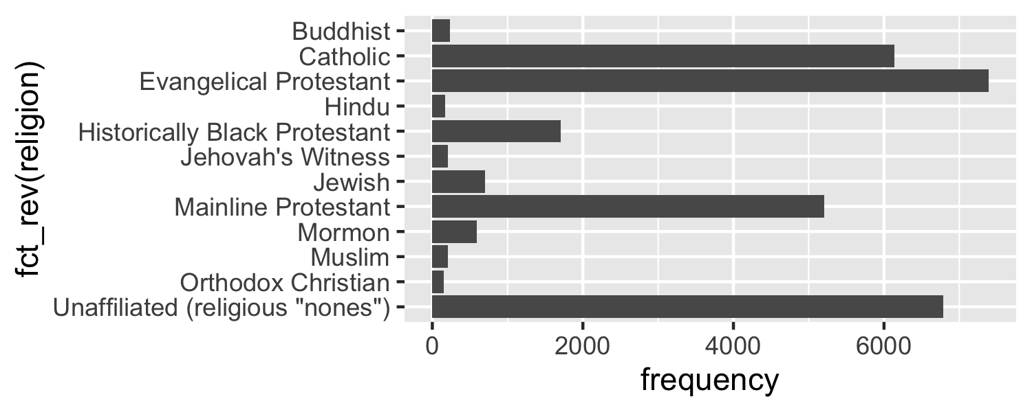
```

![](05-tidy-data_files/figure-html/unnamed-chunk-36-1.png)

---

## Add income

```r
*ggplot(rel_inc_long, aes(y = fct_rev(religion), x = frequency, fill = income)) +
  geom_col()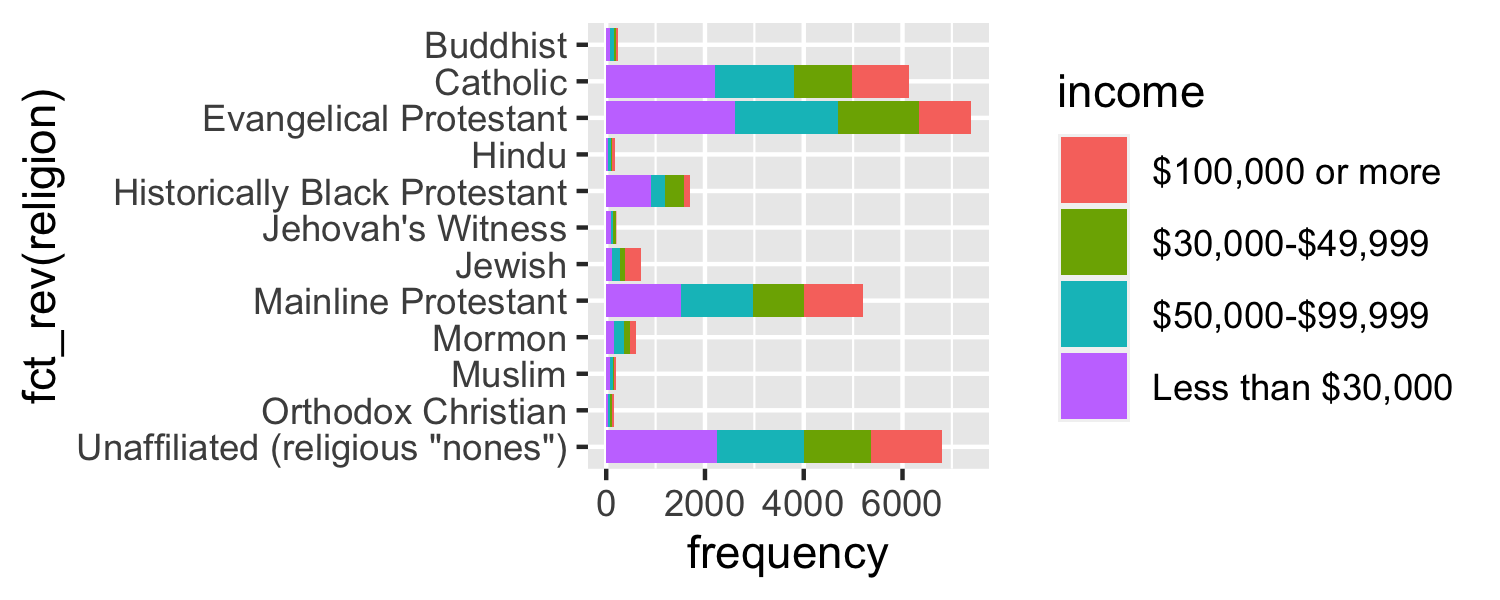 
```

![](05-tidy-data_files/figure-html/unnamed-chunk-37-1.png)

---

## Dodge bars

```r
ggplot(rel_inc_long, aes(y = fct_rev(religion), x = frequency, fill = income)) +
* geom_col(position = "dodge")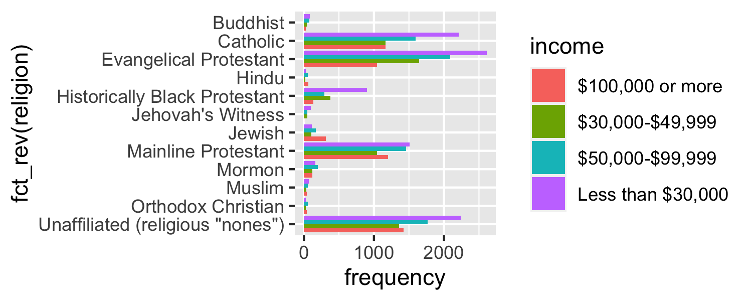
```

![](05-tidy-data_files/figure-html/unnamed-chunk-38-1.png)
]

---

## Change theme

```r
ggplot(rel_inc_long, aes(y = fct_rev(religion), x = frequency, fill = income)) +
  geom_col(position = "dodge") +
* theme_minimal()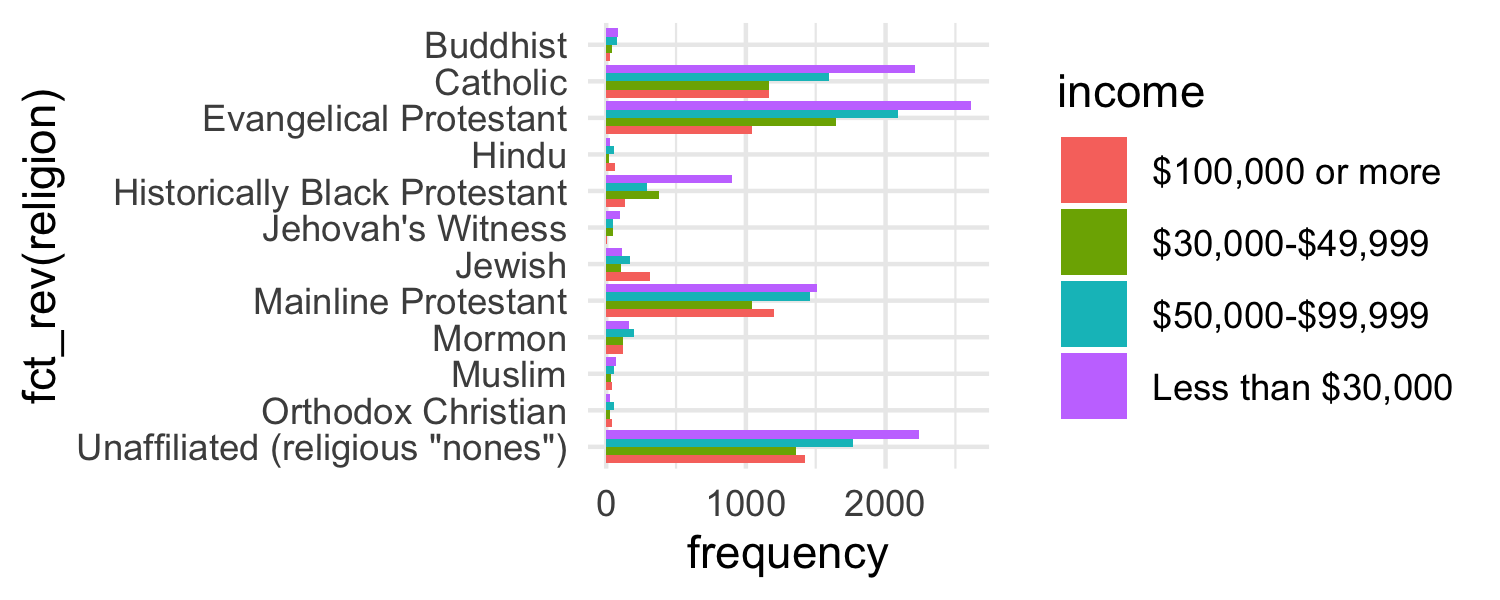
```

![](05-tidy-data_files/figure-html/unnamed-chunk-39-1.png)
]

---

## Move legend to the bottom

```r
ggplot(rel_inc_long, aes(y = fct_rev(religion), x = frequency, fill = income)) +
  geom_col(position = "dodge") +
  theme_minimal() +
* theme(legend.position = "bottom")
```

![](05-tidy-data_files/figure-html/unnamed-chunk-40-1.png)
]

---

## Prettier colors

```r
ggplot(rel_inc_long, aes(y = fct_rev(religion), x = frequency, fill = income)) +
  geom_col(position = "dodge") +
  theme_minimal() +
  theme(legend.position = "bottom") +
* scale_fill_viridis_d()
```

![](05-tidy-data_files/figure-html/unnamed-chunk-41-1.png)
]

---

## Fix labels

```r
ggplot(rel_inc_long, aes(y = fct_rev(religion), x = frequency, fill = income)) +
  geom_col(position = "dodge") +
  theme_minimal() +
  theme(legend.position = "bottom") +
  scale_fill_viridis_d() +
* labs(
*   x = "Frequency", y = "",
*   title = "Income distribution by religious group",
*   caption = "Source: pewforum.org/religious-landscape-study/income-distribution"
*   )
```

---

![](05-tidy-data_files/figure-html/unnamed-chunk-43-1.png)