class: center, middle, inverse, title-slide # Data types and recoding <br> 💽 --- layout: true <div class="my-footer"> <span> <a href="https://rstd.io/bootcamper" target="_blank">rstd.io/bootcamper</a> </span> </div> --- ## So far in bootcamper... - Took a tour through an end-to-end analysis of data from the UN General Assembly in various flavours of R Markdown - Visualized data with ggplot2 - Transformed data with dplyr - Tidied up data with tidyr .discussion[ Any questions? ] --- class: middle # Data classes and types --- ## Data types in R * **logical** * **double** * **integer** * **character** * **lists** * and some more, but we won't be focusing on those --- ## Logical & character .pull-left[ **logical** - boolean values `TRUE` and `FALSE` ```r typeof(TRUE) ``` ``` ## [1] "logical" ``` ] .pull-right[ **character** - character strings ```r typeof("hello") ``` ``` ## [1] "character" ``` ] --- ## Double & integer .pull-left[ **double** - floating point numerical values (default numerical type) ```r typeof(1.335) ``` ``` ## [1] "double" ``` ```r typeof(7) ``` ``` ## [1] "double" ``` ] .pull-right[ **integer** - integer numerical values (indicated with an `L`) ```r typeof(7L) ``` ``` ## [1] "integer" ``` ```r typeof(1:3) ``` ``` ## [1] "integer" ``` ] --- ## Lists **Lists** are 1d objects that can contain any combination of R objects .pull-left[ .midi[ ```r mylist <- list( "A", 1:4, c(TRUE, FALSE), (1:4)/2 ) mylist ``` ``` ## [[1]] ## [1] "A" ## ## [[2]] ## [1] 1 2 3 4 ## ## [[3]] ## [1] TRUE FALSE ## ## [[4]] ## [1] 0.5 1.0 1.5 2.0 ``` ] ] .pull-right[ ```r str(mylist) ``` ``` ## List of 4 ## $ : chr "A" ## $ : int [1:4] 1 2 3 4 ## $ : logi [1:2] TRUE FALSE ## $ : num [1:4] 0.5 1 1.5 2 ``` ] --- ## Named lists Because of their more complex structure we often want to name the elements of a list (we can also do this with vectors). This can make reading and accessing the list more straight forward. .pull-left[ ```r myotherlist <- list( A = "hello", B = 1:4, "knock knock" = "who's there?" ) ``` ] .pull-right[ .midi[ ```r str(myotherlist) ``` ``` ## List of 3 ## $ A : chr "hello" ## $ B : int [1:4] 1 2 3 4 ## $ knock knock: chr "who's there?" ``` ```r names(myotherlist) ``` ``` ## [1] "A" "B" "knock knock" ``` ```r myotherlist$B ``` ``` ## [1] 1 2 3 4 ``` ] ] --- ## Concatenation Vectors can be constructed using the `c()` function. ```r c(1, 2, 3) ``` ``` ## [1] 1 2 3 ``` ```r c("Hello", "World!") ``` ``` ## [1] "Hello" "World!" ``` ```r c(1, c(2, c(3))) ``` ``` ## [1] 1 2 3 ``` --- ## Vectors vs. lists .pull-left[ ```r x <- c(8,4,7) ``` ```r x[1] ``` ``` ## [1] 8 ``` ```r x[[1]] ``` ``` ## [1] 8 ``` ] -- .pull-right[ ```r y <- list(8,4,7) ``` ```r y[2] ``` ``` ## [[1]] ## [1] 4 ``` ```r y[[2]] ``` ``` ## [1] 4 ``` ] -- <br> **Note:** When using tidyverse code you'll rarely need to refer to elements using square brackets, but it's good to be aware of this syntax, especially since you might encounter it when searching for help online. --- <img src="img/hadley-salt-pepper.png" width="80%" style="display: block; margin: auto;" /> --- ## Type coercion R will happily convert between the various types without complaint. ```r c(1, "Hello") ``` ``` ## [1] "1" "Hello" ``` ```r c(FALSE, 3L) ``` ``` ## [1] 0 3 ``` ```r c(1.2, 3L) ``` ``` ## [1] 1.2 3.0 ``` -- ...and that's not alwas a great thing! --- ## Missing Values R uses `NA` to represent missing values in its data structures. ```r typeof(NA) ``` ``` ## [1] "logical" ``` --- ## `NA`s are special ❄️s ```r x <- c(1, 2, 3, 4, NA) ``` ```r mean(x) ``` ``` ## [1] NA ``` ```r mean(x, na.rm = TRUE) ``` ``` ## [1] 2.5 ``` ```r summary(x) ``` ``` ## Min. 1st Qu. Median Mean 3rd Qu. Max. NA's ## 1.00 1.75 2.50 2.50 3.25 4.00 1 ``` --- ## Other Special Values `NaN` - Not a number `Inf` - Positive infinity `-Inf` - Negative infinity -- .pull-left[ ```r pi / 0 ``` ``` ## [1] Inf ``` ```r 0 / 0 ``` ``` ## [1] NaN ``` ```r 1/0 + 1/0 ``` ``` ## [1] Inf ``` ] .pull-right[ ```r 1/0 - 1/0 ``` ``` ## [1] NaN ``` ```r NaN / NA ``` ``` ## [1] NaN ``` ```r NaN * NA ``` ``` ## [1] NaN ``` ] --- .midi[ .your-turn[ - Start the assignment titled 06 - Data types and open `01-type-coercion.Rmd`. - What is the type of the given vectors? First, guess. Then, try it out in R. If your guess was correct, great! If not, discuss why they have that type. **Strong recommendation:** One person should share their screen to facilitate discussion. ] ] .small[ **Example:** Suppose we want to know the type of `c(1, "a")`. First, I'd look at: .pull-left[ ```r typeof(1) ``` ``` ## [1] "double" ``` ] .pull-right[ ```r typeof("a") ``` ``` ## [1] "character" ``` ] and make a guess based on these. Then finally I'd check: .pull-left[ ```r typeof(c(1, "a")) ``` ``` ## [1] "character" ``` ] ] <div class="countdown" id="timer_5e98b45b" style="right:0;bottom:0;" data-warnwhen="0"> <code class="countdown-time"><span class="countdown-digits minutes">10</span><span class="countdown-digits colon">:</span><span class="countdown-digits seconds">00</span></code> </div> .footnote[ RStudio Cloud workspace for this bootcamp is at [rstd.io/bootcamper-cloud](https://rstd.io/bootcamper-cloud). ] --- ## Example: Cat lovers A survey asked respondents their name and number of cats. The instructions said to enter the number of cats as a numerical value. ```r cat_lovers <- read_csv("data/cat-lovers.csv") ``` ``` ## # A tibble: 60 x 3 ## name number_of_cats handedness ## <chr> <chr> <chr> ## 1 Bernice Warren 0 left ## 2 Woodrow Stone 0 left ## 3 Willie Bass 1 left ## 4 Tyrone Estrada 3 left ## 5 Alex Daniels 3 left ## 6 Jane Bates 2 left ## # … with 54 more rows ``` --- ## Oh why won't you work?! ```r cat_lovers %>% summarise(mean = mean(number_of_cats)) ``` ``` ## Warning in mean.default(number_of_cats): argument is not numeric or logical: returning NA ``` ``` ## # A tibble: 1 x 1 ## mean ## <dbl> ## 1 NA ``` --- ```r ?mean ``` <img src="img/mean-help.png" width="80%" style="display: block; margin: auto;" /> --- ## Oh why won't you still work??!! ```r cat_lovers %>% summarise(mean_cats = mean(number_of_cats, na.rm = TRUE)) ``` ``` ## Warning in mean.default(number_of_cats, na.rm = TRUE): argument is not numeric or logical: returning ## NA ``` ``` ## # A tibble: 1 x 1 ## mean_cats ## <dbl> ## 1 NA ``` --- ## Take a breath and look at your data .discussion[ What is the type of the `number_of_cats` variable? ] ```r glimpse(cat_lovers) ``` ``` ## Rows: 60 ## Columns: 3 ## $ name <chr> "Bernice Warren", "Woodrow Stone", "Willie Bass", "Tyrone Estrada", "Alex … ## $ number_of_cats <chr> "0", "0", "1", "3", "3", "2", "1", "1", "0", "0", "0", "0", "1", "3", "3",… ## $ handedness <chr> "left", "left", "left", "left", "left", "left", "left", "left", "left", "l… ``` --- ## Let's take another look .small[ <div id="htmlwidget-454ecd730d7db73d0383" style="width:100%;height:auto;" class="datatables html-widget"></div> <script type="application/json" data-for="htmlwidget-454ecd730d7db73d0383">{"x":{"filter":"none","data":[["1","2","3","4","5","6","7","8","9","10","11","12","13","14","15","16","17","18","19","20","21","22","23","24","25","26","27","28","29","30","31","32","33","34","35","36","37","38","39","40","41","42","43","44","45","46","47","48","49","50","51","52","53","54","55","56","57","58","59","60"],["Bernice Warren","Woodrow Stone","Willie Bass","Tyrone Estrada","Alex Daniels","Jane Bates","Latoya Simpson","Darin Woods","Agnes Cobb","Tabitha Grant","Perry Cross","Wanda Silva","Alicia Sims","Emily Logan","Woodrow Elliott","Brent Copeland","Pedro Carlson","Patsy Luna","Brett Robbins","Oliver George","Calvin Perry","Lora Gutierrez","Charlotte Sparks","Earl Mack","Leslie Wade","Santiago Barker","Jose Bell","Lynda Smith","Bradford Marshall","Irving Miller","Caroline Simpson","Frances Welch","Melba Jenkins","Veronica Morales","Juanita Cunningham","Maurice Howard","Teri Pierce","Phil Franklin","Jan Zimmerman","Leslie Price","Bessie Patterson","Ethel Wolfe","Naomi Wright","Sadie Frank","Lonnie Cannon","Tony Garcia","Darla Newton","Ginger Clark","Lionel Campbell","Florence Klein","Harriet Leonard","Terrence Harrington","Travis Garner","Doug Bass","Pat Norris","Dawn Young","Shari Alvarez","Tamara Robinson","Megan Morgan","Kara Obrien"],["0","0","1","3","3","2","1","1","0","0","0","0","1","3","3","2","1","1","0","0","1","1","0","0","4","0","0","0","0","0","0","0","0","0","0","0","0","0","0","0","0","0","1","3","3","2","1","1.5 - honestly I think one of my cats is half human","0","0","0","0","1","three","1","1","1","0","0","2"],["left","left","left","left","left","left","left","left","left","left","left","left","left","right","right","right","right","right","right","right","right","right","right","right","right","right","right","right","right","right","right","right","right","right","right","right","right","right","right","right","right","right","right","right","right","right","right","right","right","right","right","right","right","right","right","ambidextrous","ambidextrous","ambidextrous","ambidextrous","ambidextrous"]],"container":"<table class=\"display\">\n <thead>\n <tr>\n <th> <\/th>\n <th>name<\/th>\n <th>number_of_cats<\/th>\n <th>handedness<\/th>\n <\/tr>\n <\/thead>\n<\/table>","options":{"order":[],"autoWidth":false,"orderClasses":false,"columnDefs":[{"orderable":false,"targets":0}]}},"evals":[],"jsHooks":[]}</script> ] --- ## Sometimes you need to babysit your respondents ```r cat_lovers %>% mutate(number_of_cats = case_when( name == "Ginger Clark" ~ 2, name == "Doug Bass" ~ 3, TRUE ~ as.numeric(number_of_cats) )) %>% summarise(mean_cats = mean(number_of_cats)) ``` ``` ## Warning in eval_tidy(pair$rhs, env = default_env): NAs introduced by coercion ``` ``` ## # A tibble: 1 x 1 ## mean_cats ## <dbl> ## 1 0.817 ``` --- ## Always you need to respect data types ```r cat_lovers %>% mutate( number_of_cats = case_when( name == "Ginger Clark" ~ "2", name == "Doug Bass" ~ "3", TRUE ~ number_of_cats ), number_of_cats = as.numeric(number_of_cats) ) %>% summarise(mean_cats = mean(number_of_cats)) ``` ``` ## # A tibble: 1 x 1 ## mean_cats ## <dbl> ## 1 0.817 ``` --- ## Now that we know what we're doing... ```r *cat_lovers <- cat_lovers %>% mutate( number_of_cats = case_when( name == "Ginger Clark" ~ "2", name == "Doug Bass" ~ "3", TRUE ~ number_of_cats ), number_of_cats = as.numeric(number_of_cats) ) ``` --- ## Moral of the story - If your data does not behave how you expect it to, type coercion upon reading in the data might be the reason. - Go in and investigate your data, apply the fix, *save your data*, live happily ever after. --- class: middle # Data "set" --- ## Data "sets" in R - "set" is in quotation marks because it is not a formal data class -- - A tidy data "set" can be one of the following types: + `tibble` + `data.frame` -- - We'll often work with `tibble`s: + `readr` package (e.g. `read_csv` function) loads data as a `tibble` by default + `tibble`s are part of the tidyverse, so they work well with other packages we are using + they make minimal assumptions about your data, so are less likely to cause hard to track bugs in your code --- ## Data frames - A data frame is the most commonly used data structure in R: it is a list of equal length vectors. -- - Each vector is treated as a column and elements of the vectors as rows. -- - A tibble is a type of data frame that makes your life (i.e. data analysis) easier. --- ## Constructing data frames - Most often a data frame will be constructed by reading in from a file - But we can also create them from scratch. .midi[ .pull-left[ ```r df <- tibble( x = 1:3, y = c("a", "b", "c") ) class(df) ``` ``` ## [1] "tbl_df" "tbl" "data.frame" ``` ```r glimpse(df) ``` ``` ## Rows: 3 ## Columns: 2 ## $ x <int> 1, 2, 3 ## $ y <chr> "a", "b", "c" ``` ] .pull-right[ ```r df <- tribble( ~x, ~y, 1, "a", 2, "b", 3, "c" ) df ``` ``` ## # A tibble: 3 x 2 ## x y ## <dbl> <chr> ## 1 1 a ## 2 2 b ## 3 3 c ``` ] ] --- ## Working with data frames in pipelines .discussion[ How many respondents have below average number of cats? ] -- ```r mean_cats <- cat_lovers %>% summarise(mean_cats = mean(number_of_cats)) cat_lovers %>% filter(number_of_cats < mean_cats) %>% nrow() ``` ``` ## [1] 60 ``` -- .discussion[ Do you believe this number? Why, why not? ] --- ## A result of a pipeline is always a data frame ```r mean_cats ``` ``` ## # A tibble: 1 x 1 ## mean_cats ## <dbl> ## 1 0.817 ``` ```r class(mean_cats) ``` ``` ## [1] "tbl_df" "tbl" "data.frame" ``` --- ## `pull()` can be your new best friend But use it sparingly! ```r mean_cats <- cat_lovers %>% summarise(mean_cats = mean(number_of_cats)) %>% * pull() mean_cats ``` ``` ## [1] 0.8166667 ``` ```r class(mean_cats) ``` ``` ## [1] "numeric" ``` ```r cat_lovers %>% filter(number_of_cats < mean_cats) %>% nrow() ``` ``` ## [1] 33 ``` -- .pull-left[ ```r mean_cats ``` ``` ## [1] 0.8166667 ``` ] .pull-right[ ```r class(mean_cats) ``` ``` ## [1] "numeric" ``` ] --- ## to conlcude our discussion on data frames / tibbles... .pull-left[ <img src="img/tibble-part-of-tidyverse.png" width="60%" style="display: block; margin: auto;" /> ] .pull-right[ - **tibble** is also the name of the Tidyverse package that implements this data type - But you rarely need to directly load this package since `library(tidyverse)` takes care of it - And you rarely need to use functions from this package for data wrangling and visualisation, except when you're manually creating your data frames for a short example with `tibble()` or `tribble()` ] --- ## Recap - Always best to think of data as part of a tibble + This plays nicely with the `tidyverse` as well + Rows are observations, columns are variables -- - Be careful about data types / classes + Sometimes `R` makes silly assumptions about your data class + Using `tibble`s help, but it might not solve all issues + Think about your data in context, e.g. 0/1 variable is most likely a `factor` + If a plot/output is not behaving the way you expect, first investigate the data class + If you are absolutely sure of a data class, overwrite it in your tibble so that you don't need to keep having to keep track of it + `mutate` the variable with the correct class --- ## Two data types worth knowing your way around .pull-right[ .huge-blue[factors] ] .pull-left[ .huge-blue[dates] ] --- class: middle # Factors --- ## Factors Factor objects are how R stores data for categorical variables (fixed numbers of discrete values). ```r (x = factor(c("BS", "MS", "PhD", "MS"))) ``` ``` ## [1] BS MS PhD MS ## Levels: BS MS PhD ``` ```r glimpse(x) ``` ``` ## Factor w/ 3 levels "BS","MS","PhD": 1 2 3 2 ``` ```r typeof(x) ``` ``` ## [1] "integer" ``` --- ## Read data in as character strings ```r glimpse(cat_lovers) ``` ``` ## Rows: 60 ## Columns: 3 ## $ name <chr> "Bernice Warren", "Woodrow Stone", "Willie Bass", "Tyrone Estrada", "Alex … ## $ number_of_cats <dbl> 0, 0, 1, 3, 3, 2, 1, 1, 0, 0, 0, 0, 1, 3, 3, 2, 1, 1, 0, 0, 1, 1, 0, 0, 4,… ## $ handedness <chr> "left", "left", "left", "left", "left", "left", "left", "left", "left", "l… ``` --- ## But coerce when plotting ```r ggplot(cat_lovers, mapping = aes(x = handedness)) + geom_bar() ``` <img src="06-data-types_files/figure-html/unnamed-chunk-52-1.png" width="70%" /> --- ## Use forcats to manipulate factors ```r cat_lovers %>% * mutate(handedness = fct_infreq(handedness)) %>% ggplot(mapping = aes(x = handedness)) + geom_bar() ``` <img src="06-data-types_files/figure-html/unnamed-chunk-53-1.png" width="1800" /> --- ## Come for the functionality .pull-left[ ... stay for the logo ] .pull-right[ <img src="img/forcats-part-of-tidyverse.png" width="70%" /> ] - R uses factors to handle categorical variables, variables that have a fixed and known set of possible values - Factors are useful when you have true categorical data and you want to override the ordering of character vectors to improve display - They are also useful in modeling scenarios - The **forcats** package provides a suite of useful tools that solve common problems with factors --- .your-turn[ - Start the assignment titled 06 - Data types and open `02-forcats.Rmd`. - Recreate the following -- first, the x-axis, and then, as a stretch goal, the y-axis. ] 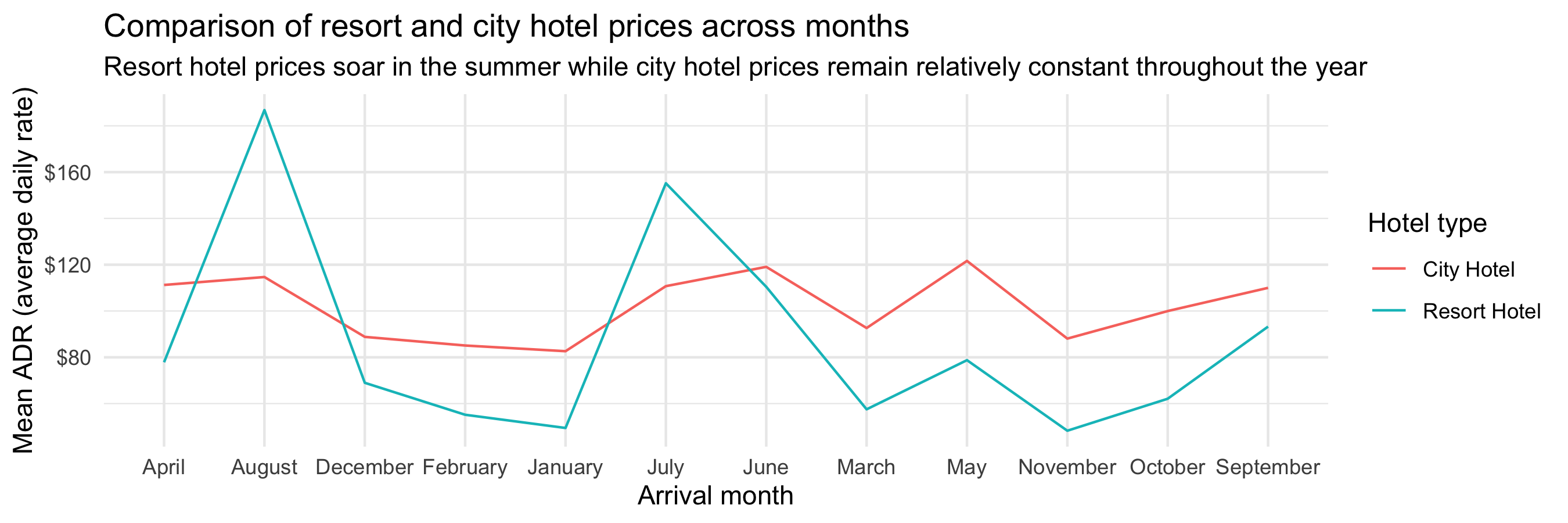<!-- --> <div class="countdown" id="timer_5e98b3e4" style="right:0;bottom:0;" data-warnwhen="0"> <code class="countdown-time"><span class="countdown-digits minutes">05</span><span class="countdown-digits colon">:</span><span class="countdown-digits seconds">00</span></code> </div> .footnote[ RStudio Cloud workspace for this bootcamp is at [rstd.io/bootcamper-cloud](https://rstd.io/bootcamper-cloud). ] --- class: middle # Dates --- ## Come for the functionality .pull-left[ <img src="img/lubridate-not-part-of-tidyverse.png" width="70%" style="display: block; margin: auto;" /> ] .pull-right[ - **lubridate** is the tidyverse-friendly package that makes dealing with dates a little easier - It's not one of the *core* tidyverse packages, hence it's installed with `install.packages("tidyverse)` but it's not loaded with it, and needs to be explicitly loaded with `library(lubridate)` ] --- class: middle .hand-blue[ we're just going to scratch the surface of working with dates in R here... ] --- .discussion[ Calculate and visualise the number of bookings on any given arrival date. ] ```r hotels %>% select(starts_with("arrival_")) ``` ``` ## # A tibble: 119,390 x 4 ## arrival_date_year arrival_date_month arrival_date_week_number arrival_date_day_of_month ## <dbl> <chr> <dbl> <dbl> ## 1 2015 July 27 1 ## 2 2015 July 27 1 ## 3 2015 July 27 1 ## 4 2015 July 27 1 ## 5 2015 July 27 1 ## 6 2015 July 27 1 ## # … with 119,384 more rows ``` --- ### Step 1. Put together dates. .midi[ ```r library(glue) hotels %>% mutate( * arrival_date = glue("{arrival_date_year} {arrival_date_month} {arrival_date_day_of_month}") ) %>% select(starts_with("arrival_")) ``` ``` ## # A tibble: 119,390 x 5 ## arrival_date_year arrival_date_month arrival_date_week_numb… arrival_date_day_of_mon… arrival_date ## <dbl> <chr> <dbl> <dbl> <glue> ## 1 2015 July 27 1 2015 July 1 ## 2 2015 July 27 1 2015 July 1 ## 3 2015 July 27 1 2015 July 1 ## 4 2015 July 27 1 2015 July 1 ## 5 2015 July 27 1 2015 July 1 ## 6 2015 July 27 1 2015 July 1 ## # … with 119,384 more rows ``` ] --- ### Step 2. Count number of bookings per date. .midi[ ```r hotels %>% mutate(arrival_date = glue("{arrival_date_year} {arrival_date_month} {arrival_date_day_of_month}")) %>% count(arrival_date) ``` ``` ## # A tibble: 793 x 2 ## arrival_date n ## * <glue> <int> ## 1 2015 August 1 110 ## 2 2015 August 10 207 ## 3 2015 August 11 117 ## 4 2015 August 12 133 ## 5 2015 August 13 107 ## 6 2015 August 14 329 ## # … with 787 more rows ``` ] --- ### Step 3. Visualise number of bookings per date. .midi[ ```r hotels %>% mutate(arrival_date = glue("{arrival_date_year} {arrival_date_month} {arrival_date_day_of_month}")) %>% count(arrival_date) %>% ggplot(aes(x = arrival_date, y = n, group = 1)) + geom_line() + ylim(0, 450) ``` 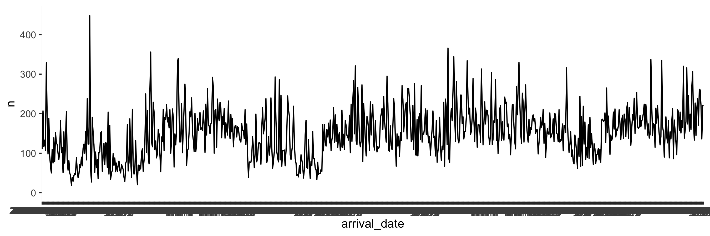<!-- --> ] --- .hand[zooming in a bit...] .question[ Why does the plot start with August when we know our data start in July? And why does 10 August come after 1 August? ] .midi[ 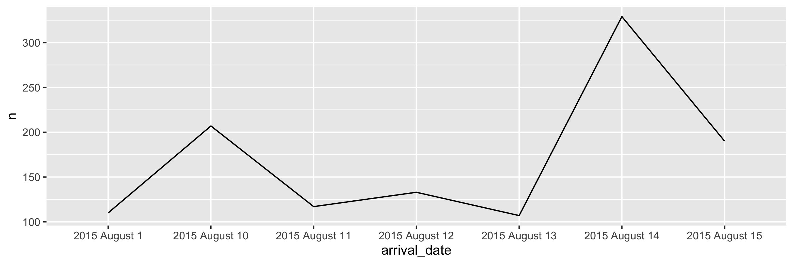<!-- --> ] --- ### Step 1. `REVISED` Put together dates `as dates`. .midi[ ```r library(lubridate) hotels %>% mutate( * arrival_date = ymd(glue("{arrival_date_year} {arrival_date_month} {arrival_date_day_of_month}")) ) %>% select(starts_with("arrival_")) ``` ``` ## # A tibble: 119,390 x 5 ## arrival_date_year arrival_date_month arrival_date_week_numb… arrival_date_day_of_mon… arrival_date ## <dbl> <chr> <dbl> <dbl> <date> ## 1 2015 July 27 1 2015-07-01 ## 2 2015 July 27 1 2015-07-01 ## 3 2015 July 27 1 2015-07-01 ## 4 2015 July 27 1 2015-07-01 ## 5 2015 July 27 1 2015-07-01 ## 6 2015 July 27 1 2015-07-01 ## # … with 119,384 more rows ``` ] --- ### Step 2. Count number of bookings per date. .midi[ ```r hotels %>% mutate(arrival_date = ymd(glue("{arrival_date_year} {arrival_date_month} {arrival_date_day_of_month}"))) %>% count(arrival_date) ``` ``` ## # A tibble: 793 x 2 ## arrival_date n ## * <date> <int> ## 1 2015-07-01 122 ## 2 2015-07-02 93 ## 3 2015-07-03 56 ## 4 2015-07-04 88 ## 5 2015-07-05 53 ## 6 2015-07-06 75 ## # … with 787 more rows ``` ] --- ### Step 3a. Visualise number of bookings per date. .midi[ ```r hotels %>% mutate(arrival_date = ymd(glue("{arrival_date_year} {arrival_date_month} {arrival_date_day_of_month}"))) %>% count(arrival_date) %>% ggplot(aes(x = arrival_date, y = n, group = 1)) + geom_line() + ylim(0, 450) ``` 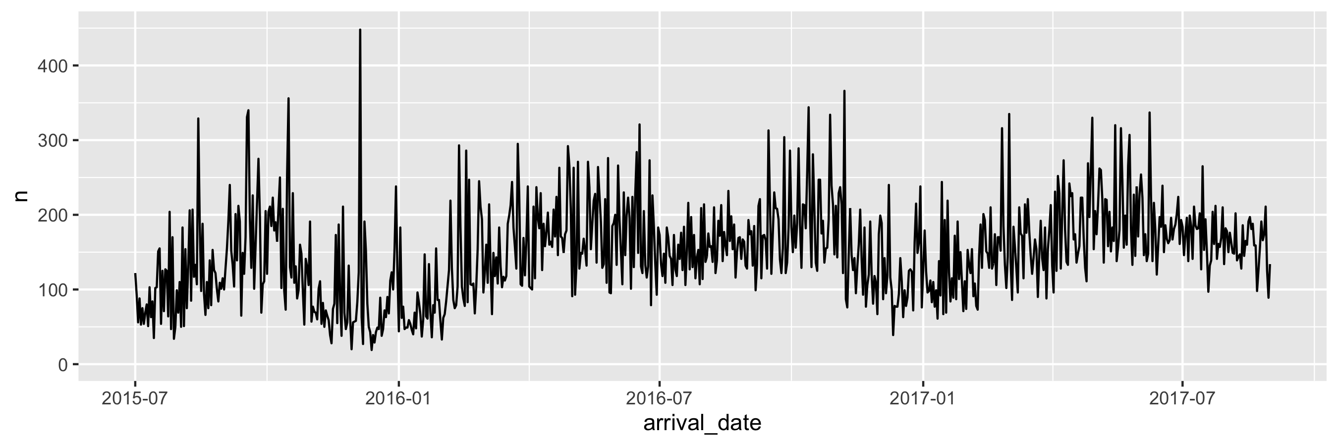<!-- --> ] --- ### Step 3b. Visualise number of bookings per date, using a smooth curve. .midi[ ```r hotels %>% mutate(arrival_date = ymd(glue("{arrival_date_year} {arrival_date_month} {arrival_date_day_of_month}"))) %>% count(arrival_date) %>% ggplot(aes(x = arrival_date, y = n, group = 1)) + * geom_smooth() + ylim(0, 450) ``` 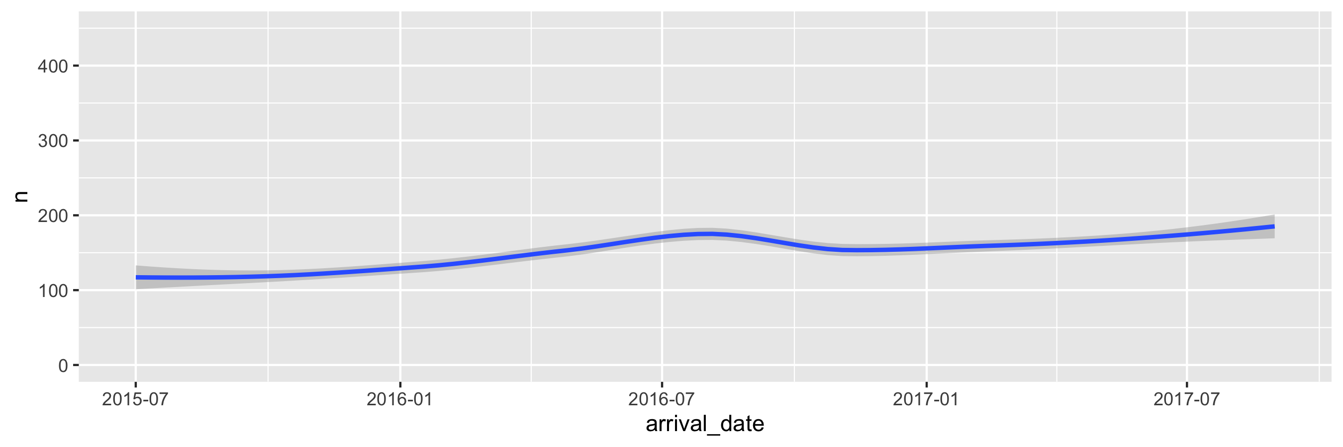<!-- --> ]