12 Speed
As a data scientist, you need speed. You can work with bigger data and do more ambitious tasks when your code runs fast. This chapter will show you a specific way to write fast code in R. You will then use the method to simulate 10 million plays of your slot machine.
12.1 Vectorized Code
You can write a piece of code in many different ways, but the fastest R code will usually take advantage of three things: logical tests, subsetting, and element-wise execution. These are the things that R does best. Code that uses these things usually has a certain quality: it is vectorized; the code can take a vector of values as input and manipulate each value in the vector at the same time.
To see what vectorized code looks like, compare these two examples of an absolute value function. Each takes a vector of numbers and transforms it into a vector of absolute values (e.g., positive numbers). The first example is not vectorized; abs_loop uses a for loop to manipulate each element of the vector one at a time:
abs_loop <- function(vec){
  for (i in 1:length(vec)) {
    if (vec[i] < 0) {
      vec[i] <- -vec[i]
    }
  }
  vec
}
The second example, abs_set, is a vectorized version of abs_loop. It uses logical subsetting to manipulate every negative number in the vector at the same time:
abs_sets <- function(vec){
  negs <- vec < 0
  vec[negs] <- vec[negs] * -1
  vec
}
abs_set is much faster than abs_loop because it relies on operations that R does quickly: logical tests, subsetting, and element-wise execution.
You can use the system.time function to see just how fast abs_set is. system.time takes an R expression, runs it, and then displays how much time elapsed while the expression ran.
To compare abs_loop and abs_set, first make a long vector of positive and negative numbers. long will contain 10 million values:
long <- rep(c(-1, 1), 5000000)rep repeats a value, or vector of values, many times. To use rep, give it a vector of values and then the number of times to repeat the vector. R will return the results as a new, longer vector.
You can then use system.time to measure how much time it takes each function to evaluate long:
system.time(abs_loop(long))
##    user  system elapsed
##  15.982   0.032  16.018

system.time(abs_sets(long))
##    user  system elapsed
## 0.529 0.063 0.592system.time with Sys.time, which returns the current time.
The first two columns of the output of system.time report how many seconds your computer spent executing the call on the user side and system sides of your process, a dichotomy that will vary from OS to OS.
The last column displays how many seconds elapsed while R ran the expression. The results show that abs_set calculated the absolute value 30 times faster than abs_loop when applied to a vector of 10 million numbers. You can expect similar speed-ups whenever you write vectorized code.
abs.
Check to see how much faster abs computes the absolute value of long than abs_loop and abs_set do.
abs with system.time. It takes abs a lightning-fast 0.05 seconds to calculate the absolute value of 10 million numbers. This is 0.592 / 0.054 = 10.96 times faster than abs_set and nearly 300 times faster than abs_loop:
system.time(abs(long))
##   user  system elapsed
##  0.037   0.018   0.054
12.2 How to Write Vectorized Code
Vectorized code is easy to write in R because most R functions are already vectorized. Code based on these functions can easily be made vectorized and therefore fast. To create vectorized code:
- Use vectorized functions to complete the sequential steps in your program.
- Use logical subsetting to handle parallel cases. Try to manipulate every element in a case at once.
abs_loop and abs_set illustrate these rules. The functions both handle two cases and perform one sequential step, Figure 12.1. If a number is positive, the functions leave it alone. If a number is negative, the functions multiply it by negative one.
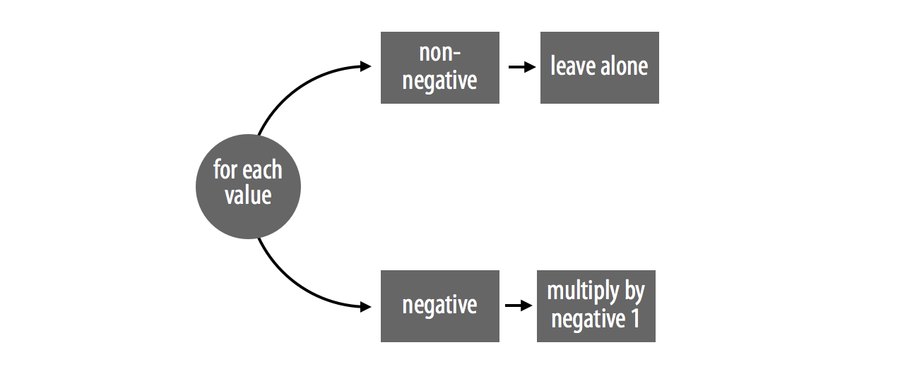
Figure 12.1: abs_loop uses a for loop to sift data into one of two cases: negative numbers and nonnegative numbers.
You can identify all of the elements of a vector that fall into a case with a logical test. R will execute the test in element-wise fashion and return a TRUE for every element that belongs in the case. For example, vec < 0 identifies every value of vec that belongs to the negative case. You can use the same logical test to extract the set of negative values with logical subsetting:
vec <- c(1, -2, 3, -4, 5, -6, 7, -8, 9, -10)
vec < 0
## FALSE TRUE FALSE TRUE FALSE TRUE FALSE TRUE FALSE TRUE

vec[vec < 0]
## -2  -4  -6  -8 -10
The plan in Figure 12.1 now requires a sequential step: you must multiply each of the negative values by negative one. All of R’s arithmetic operators are vectorized, so you can use * to complete this step in vectorized fashion. * will multiply each number in vec[vec < 0] by negative one at the same time:
vec[vec < 0] * -1
## 2  4  6  8 10
Finally, you can use R’s assignment operator, which is also vectorized, to save the new set over the old set in the original vec object. Since <- is vectorized, the elements of the new set will be paired up to the elements of the old set, in order, and then element-wise assignment will occur. As a result, each negative value will be replaced by its positive partner, as in Figure 12.2.
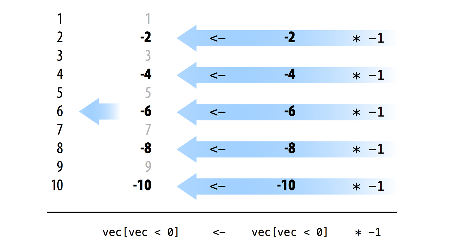
Figure 12.2: Use logical subsetting to modify groups of values in place. R’s arithmetic and assignment operators are vectorized, which lets you manipulate and update multiple values at once.
change_symbols <- function(vec){
  for (i in 1:length(vec)){
    if (vec[i] == "DD") {
      vec[i] <- "joker"
    } else if (vec[i] == "C") {
      vec[i] <- "ace"
    } else if (vec[i] == "7") {
      vec[i] <- "king"
    }else if (vec[i] == "B") {
      vec[i] <- "queen"
    } else if (vec[i] == "BB") {
      vec[i] <- "jack"
    } else if (vec[i] == "BBB") {
      vec[i] <- "ten"
    } else {
      vec[i] <- "nine"
    }
  }
  vec
}

vec <- c("DD", "C", "7", "B", "BB", "BBB", "0")

change_symbols(vec)
##  "joker" "ace"   "king"  "queen" "jack"  "ten"   "nine"

many <- rep(vec, 1000000)

system.time(change_symbols(many))
##    user  system elapsed
## 30.057 0.031 30.079change_symbols uses a for loop to sort values into seven different cases, as demonstrated in Figure 12.3.
To vectorize change_symbols, create a logical test that can identify each case:
vec[vec == "DD"]
## "DD"

vec[vec == "C"]
## "C"

vec[vec == "7"]
## "7"

vec[vec == "B"]
## "B"

vec[vec == "BB"]
## "BB"

vec[vec == "BBB"]
## "BBB"

vec[vec == "0"]
## "0"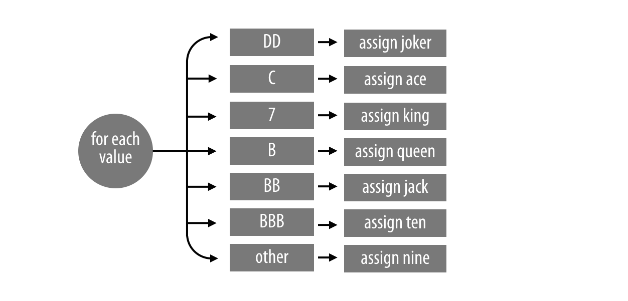
Figure 12.3: change_many does something different for each of seven cases.
Then write code that can change the symbols for each case:
vec[vec == "DD"] <- "joker"
vec[vec == "C"] <- "ace"
vec[vec == "7"] <- "king"
vec[vec == "B"] <- "queen"
vec[vec == "BB"] <- "jack"
vec[vec == "BBB"] <- "ten"
vec[vec == "0"] <- "nine"
When you combine this into a function, you have a vectorized version of change_symbols that runs about 14 times faster:
change_vec <- function (vec) {
  vec[vec == "DD"] <- "joker"
  vec[vec == "C"] <- "ace"
  vec[vec == "7"] <- "king"
  vec[vec == "B"] <- "queen"
  vec[vec == "BB"] <- "jack"
  vec[vec == "BBB"] <- "ten"
  vec[vec == "0"] <- "nine"

  vec
}

system.time(change_vec(many))
##   user  system elapsed
##  1.994   0.059   2.051
Or, even better, use a lookup table. Lookup tables are a vectorized method because they rely on R’s vectorized selection operations:
change_vec2 <- function(vec){
  tb <- c("DD" = "joker", "C" = "ace", "7" = "king", "B" = "queen",
    "BB" = "jack", "BBB" = "ten", "0" = "nine")
  unname(tb[vec])
}

system.time(change_vec(many))
##   user  system elapsed
##  0.687   0.059   0.746
Here, a lookup table is 40 times faster than the original function.
abs_loop and change_many illustrate a characteristic of vectorized code: programmers often write slower, nonvectorized code by relying on unnecessary for loops, like the one in change_many. I think this is the result of a general misunderstanding about R. for loops do not behave the same way in R as they do in other languages, which means you should write code differently in R than you would in other languages.
When you write in languages like C and Fortran, you must compile your code before your computer can run it. This compilation step optimizes how the for loops in the code use your computer’s memory, which makes the for loops very fast. As a result, many programmers use for loops frequently when they write in C and Fortran.
When you write in R, however, you do not compile your code. You skip this step, which makes programming in R a more user-friendly experience. Unfortunately, this also means you do not give your loops the speed boost they would receive in C or Fortran. As a result, your loops will run slower than the other operations we have studied: logical tests, subsetting, and element-wise execution. If you can write your code with the faster operations instead of a for loop, you should do so. No matter which language you write in, you should try to use the features of the language that run the fastest.
if and for
A good way to spotfor loops that could be vectorized is to look for combinations of if and for. if can only be applied to one value at a time, which means it is often used in conjunction with a for loop. The for loop helps apply if to an entire vector of values. This combination can usually be replaced with logical subsetting, which will do the same thing but run much faster.
This doesn’t mean that you should never use for loops in R. There are still many places in R where for loops make sense. for loops perform a basic task that you cannot always recreate with vectorized code. for loops are also easy to understand and run reasonably fast in R, so long as you take a few precautions.
12.3 How to Write Fast for Loops in R
You can dramatically increase the speed of your for loops by doing two things to optimize each loop. First, do as much as you can outside of the for loop. Every line of code that you place inside of the for loop will be run many, many times. If a line of code only needs to be run once, place it outside of the loop to avoid repetition.
Second, make sure that any storage objects that you use with the loop are large enough to contain all of the results of the loop. For example, both loops below will need to store one million values. The first loop stores its values in an object named output that begins with a length of one million:
system.time({
  output <- rep(NA, 1000000)
  for (i in 1:1000000) {
    output[i] <- i + 1
  }
})
##   user  system elapsed
##  1.709   0.015   1.724
The second loop stores its values in an object named output that begins with a length of one. R will expand the object to a length of one million as it runs the loop. The code in this loop is very similar to the code in the first loop, but the loop takes 37 minutes longer to run than the first loop:
system.time({
  output <- NA
  for (i in 1:1000000) {
    output[i] <- i + 1
  }
})
##     user   system  elapsed
## 1689.537  560.951 2249.927
The two loops do the same thing, so what accounts for the difference? In the second loop, R has to increase the length of output by one for each run of the loop. To do this, R needs to find a new place in your computer’s memory that can contain the larger object. R must then copy the output vector over and erase the old version of output before moving on to the next run of the loop. By the end of the loop, R has rewritten output in your computer’s memory one million times.
In the first case, the size of output never changes; R can define one output object in memory and use it for each run of the for loop.
The authors of R use low-level languages like C and Fortran to write basic R functions, many of which use for loops. These functions are compiled and optimized before they become a part of R, which makes them quite fast.
.Primitive, .Internal, or .Call written in a function’s definition, you can be confident the function is calling code from another language. You’ll get all of the speed advantages of that language by using the function.
12.4 Vectorized Code in Practice
To see how vectorized code can help you as a data scientist, consider our slot machine project. In Loops, you calculated the exact payout rate for your slot machine, but you could have estimated this payout rate with a simulation. If you played the slot machine many, many times, the average prize over all of the plays would be a good estimate of the true payout rate.
This method of estimation is based on the law of large numbers and is similar to many statistical simulations. To run this simulation, you could use a for loop:
winnings <- vector(length = 1000000)
for (i in 1:1000000) {
  winnings[i] <- play()
}

mean(winnings)
## 0.9366984
The estimated payout rate after 10 million runs is 0.937, which is very close to the true payout rate of 0.934. Note that I’m using the modified score function that treats diamonds as wilds.
If you run this simulation, you will notice that it takes a while to run. In fact, the simulation takes 342,308 seconds to run, which is about 5.7 minutes. This is not particularly impressive, and you can do better by using vectorized code:
system.time(for (i in 1:1000000) {
  winnings[i] <- play()
})
##    user  system elapsed
## 342.041   0.355 342.308
The current score function is not vectorized. It takes a single slot combination and uses an if tree to assign a prize to it. This combination of an if tree with a for loop suggests that you could write a piece of vectorized code that takes many slot combinations and then uses logical subsetting to operate on them all at once.
For example, you could rewrite get_symbols to generate n slot combinations and return them as an n x 3 matrix, like the one that follows. Each row of the matrix will contain one slot combination to be scored:
get_many_symbols <- function(n) {
  wheel <- c("DD", "7", "BBB", "BB", "B", "C", "0")
  vec <- sample(wheel, size = 3 * n, replace = TRUE,
    prob = c(0.03, 0.03, 0.06, 0.1, 0.25, 0.01, 0.52))
  matrix(vec, ncol = 3)
}

get_many_symbols(5)
##      [,1]  [,2] [,3]
## [1,] "B"   "0"  "B"
## [2,] "0"   "BB" "7"
## [3,] "0"   "0"  "BBB"
## [4,] "0"   "0"  "B"
## [5,] "BBB" "0"  "0"
You could also rewrite play to take a parameter, n, and return n prizes, in a data frame:
play_many <- function(n) {
  symb_mat <- get_many_symbols(n = n)
  data.frame(w1 = symb_mat[,1], w2 = symb_mat[,2],
             w3 = symb_mat[,3], prize = score_many(symb_mat))
}
This new function would make it easy to simulate a million, or even 10 million plays of the slot machine, which will be our goal. When we’re finished, you will be able to estimate the payout rate with:
# plays <- play_many(10000000))
# mean(plays$prize)
Now you just need to write score_many, a vectorized (matix-ized?) version of score that takes an n x 3 matrix and returns n prizes. It will be difficult to write this function because score is already quite complicated. I would not expect you to feel confident doing this on your own until you have more practice and experience than we’ve been able to develop here.
Should you like to test your skills and write a version of score_many, I recommend that you use the function rowSums within your code. It calculates the sum of each row of numbers (or logicals) in a matrix.
If you would like to test yourself in a more modest way, I recommend that you study the following model score_many function until you understand how each part works and how the parts work together to create a vectorized function. To do this, it will be helpful to create a concrete example, like this:
symbols <- matrix(
  c("DD", "DD", "DD",
    "C", "DD", "0",
    "B", "B", "B",
    "B", "BB", "BBB",
    "C", "C", "0",
    "7", "DD", "DD"), nrow = 6, byrow = TRUE)

symbols
##      [,1] [,2] [,3]
## [1,] "DD" "DD" "DD"
## [2,] "C"  "DD" "0"
## [3,] "B"  "B"  "B"
## [4,] "B"  "BB" "BBB"
## [5,] "C"  "C"  "0"
## [6,] "7"  "DD" "DD"
Then you can run each line of score_many against the example and examine the results as you go.
score_many function until you are satisfied that you understand how it works and could write a similar function yourself.
score. Assume that the data is stored in an n × 3 matrix where each row of the matrix contains one combination of slots to be scored.
You can use the version of score that treats diamonds as wild or the version of score that doesn’t. However, the model answer will use the version treating diamonds as wild.
score_many is a vectorized version of score. You can use it to run the simulation at the start of this section in a little over 20 seconds. This is 17 times faster than using a for loop:
# symbols should be a matrix with a column for each slot machine window
score_many <- function(symbols) {

  # Step 1: Assign base prize based on cherries and diamonds ---------
  ## Count the number of cherries and diamonds in each combination
  cherries <- rowSums(symbols == "C")
  diamonds <- rowSums(symbols == "DD")

  ## Wild diamonds count as cherries
  prize <- c(0, 2, 5)[cherries + diamonds + 1]

  ## ...but not if there are zero real cherries
  ### (cherries is coerced to FALSE where cherries == 0)
  prize[!cherries] <- 0

  # Step 2: Change prize for combinations that contain three of a kind
  same <- symbols[, 1] == symbols[, 2] &
    symbols[, 2] == symbols[, 3]
  payoffs <- c("DD" = 100, "7" = 80, "BBB" = 40,
    "BB" = 25, "B" = 10, "C" = 10, "0" = 0)
  prize[same] <- payoffs[symbols[same, 1]]

  # Step 3: Change prize for combinations that contain all bars ------
  bars <- symbols == "B" | symbols ==  "BB" | symbols == "BBB"
  all_bars <- bars[, 1] & bars[, 2] & bars[, 3] & !same
  prize[all_bars] <- 5

  # Step 4: Handle wilds ---------------------------------------------

  ## combos with two diamonds
  two_wilds <- diamonds == 2

  ### Identify the nonwild symbol
  one <- two_wilds & symbols[, 1] != symbols[, 2] &
    symbols[, 2] == symbols[, 3]
  two <- two_wilds & symbols[, 1] != symbols[, 2] &
    symbols[, 1] == symbols[, 3]
  three <- two_wilds & symbols[, 1] == symbols[, 2] &
    symbols[, 2] != symbols[, 3]

  ### Treat as three of a kind
  prize[one] <- payoffs[symbols[one, 1]]
  prize[two] <- payoffs[symbols[two, 2]]
  prize[three] <- payoffs[symbols[three, 3]]

  ## combos with one wild
  one_wild <- diamonds == 1

  ### Treat as all bars (if appropriate)
  wild_bars <- one_wild & (rowSums(bars) == 2)
  prize[wild_bars] <- 5

  ### Treat as three of a kind (if appropriate)
  one <- one_wild & symbols[, 1] == symbols[, 2]
  two <- one_wild & symbols[, 2] == symbols[, 3]
  three <- one_wild & symbols[, 3] == symbols[, 1]
  prize[one] <- payoffs[symbols[one, 1]]
  prize[two] <- payoffs[symbols[two, 2]]
  prize[three] <- payoffs[symbols[three, 3]]

  # Step 5: Double prize for every diamond in combo ------------------
  unname(prize * 2^diamonds)

}

system.time(play_many(10000000))
##   user  system elapsed
## 20.942   1.433  22.367
12.4.1 Loops Versus Vectorized Code
In many languages, for loops run very fast. As a result, programmers learn to use for loops whenever possible when they code. Often these programmers continue to rely on for loops when they begin to program in R, usually without taking the simple steps needed to optimize R’s for loops. These programmers may become disillusioned with R when their code does not work as fast as they would like. If you think that this may be happening to you, examine how often you are using for loops and what you are using them to do. If you find yourself using for loops for every task, there is a good chance that you are “speaking R with a C accent.” The cure is to learn to write and use vectorized code.
This doesn’t mean that for loops have no place in R. for loops are a very useful feature; they can do many things that vectorized code cannot do. You also should not become a slave to vectorized code. Sometimes it would take more time to rewrite code in vectorized format than to let a for loop run. For example, would it be faster to let the slot simulation run for 5.7 minutes or to rewrite score?
12.5 Summary
Fast code is an important component of data science because you can do more with fast code than you can do with slow code. You can work with larger data sets before computational constraints intervene, and you can do more computation before time constraints intervene. The fastest code in R will rely on the things that R does best: logical tests, subsetting, and element-wise execution. I’ve called this type of code vectorized code because code written with these operations will take a vector of values as input and operate on each element of the vector at the same time. The majority of the code written in R is already vectorized.
If you use these operations, but your code does not appear vectorized, analyze the sequential steps and parallel cases in your program. Ensure that you’ve used vectorized functions to handle the steps and logical subsetting to handle the cases. Be aware, however, that some tasks cannot be vectorized.
12.6 Project 3 Wrap-up
You have now written your first program in R, and it is a program that you should be proud of. play is not a simple hello world exercise, but a real program that does a real task in a complicated way.
Writing new programs in R will always be challenging because programming depends so much on your own creativity, problem-solving ability, and experience writing similar types of programs. However, you can use the suggestions in this chapter to make even the most complicated program manageable: divide tasks into simple steps and cases, work with concrete examples, and describe possible solutions in English.
This project completes the education you began in The Very Basics. You can now use R to handle data, which has augmented your ability to analyze data. You can:
- Load and store data in your computer—not on paper or in your mind
- Accurately recall and change individual values without relying on your memory
- Instruct your computer to do tedious, or complex, tasks on your behalf
These skills solve an important logistical problem faced by every data scientist: how can you store and manipulate data without making errors? However, this is not the only problem that you will face as a data scientist. The next problem will appear when you try to understand the information contained in your data. It is nearly impossible to spot insights or to discover patterns in raw data. A third problem will appear when you try to use your data set to reason about reality, which includes things not contained in your data set. What exactly does your data imply about things outside of the data set? How certain can you be?
I refer to these problems as the logistical, tactical, and strategic problems of data science, as shown in Figure 12.4. You’ll face them whenever you try to learn from data:
- A logistical problem: - How can you store and manipulate data without making errors?
- A tactical problem - How can you discover the information contained in your data?
- A strategic problem - How can you use the data to draw conclusions about the world at large?
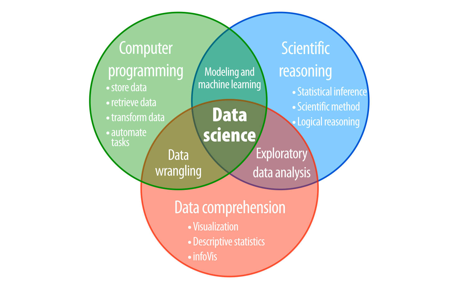
Figure 12.4: The three core skill sets of data science: computer programming, data comprehension, and scientific reasoning.
A well-rounded data scientist will need to be able to solve each of these problems in many different situations. By learning to program in R, you have mastered the logistical problem, which is a prerequisite for solving the tactical and strategic problems.
If you would like to learn how to reason with data, or how to transform, visualize, and explore your data sets with R tools, I recommend the book R for Data Science, the companion volume to this book. R for Data Science teaches a simple workflow for transforming, visualizing, and modeling data in R, as well as how to report results with the R Markdown package.