3 Tidy
This chapter includes the following recipes:
- Create a tibble manually
- Convert a data frame to a tibble
- Convert a tibble to a data frame
- Preview the contents of a tibble
- Inspect every cell of a tibble
- Spread a pair of columns into a field of cells
- Gather a field of cells into a pair of columns
- Separate a column into new columns
- Unite multiple columns into a single column
What you should know before you begin
Data tidying refers to reshaping your data into a tidy data frame or tibble. Data tidying is an important first step for your analysis because every tidyverse function will expect your data to be stored as Tidy Data.
Tidy data is tabular data organized so that:
- Each column contains a single variable
- Each row contains a single observation
Tidy data is not an arbitrary requirement of the tidyverse; it is the ideal data format for doing data science with R. Tidy data makes it easy to extract every value of a variable to build a plot or to compute a summary statistic. Tidy data also makes it easy to compute new variables; when your data is tidy, you can rely on R’s rowwise operations to maintain the integrity of your observations. Moreover, R can directly manipulate tidy data with R’s fast, built-in vectorised observations, which lets your code run as fast as possible.
The definition of Tidy Data isn’t complete until you define variable and observation, so let’s borrow two definitions from R for Data Science:
- A variable is a quantity, quality, or property that you can measure.
- An observation is a set of measurements made under similar conditions (you usually make all of the measurements in an observation at the same time and on the same object).
3.1 Create a tibble manually
You want to create a tibble from scratch by typing in the contents of the tibble.
Solution
## # A tibble: 3 x 3
##   number letter greek
##    <dbl> <chr>  <chr>
## 1      1 a      alpha
## 2      2 b      beta
## 3      3 c      gamma
Discussion
tribble() creates a tibble and tricks you into typing out a preview of the result. To use tribble(), list each column name preceded by a ~, then list the values of the tribble in a rowwise fashion. If you take care to align your columns, the transposed syntax of tribble() becomes a preview of the table.
You can also create a tibble with tibble(), whose syntax mirrors data.frame():
3.2 Convert a data frame to a tibble
You want to convert a data frame to a tibble.
Solution
## # A tibble: 150 x 5
##    Sepal.Length Sepal.Width Petal.Length Petal.Width Species
##           <dbl>       <dbl>        <dbl>       <dbl> <fct>
##  1          5.1         3.5          1.4         0.2 setosa
##  2          4.9         3            1.4         0.2 setosa
##  3          4.7         3.2          1.3         0.2 setosa
##  4          4.6         3.1          1.5         0.2 setosa
##  5          5           3.6          1.4         0.2 setosa
##  6          5.4         3.9          1.7         0.4 setosa
##  7          4.6         3.4          1.4         0.3 setosa
##  8          5           3.4          1.5         0.2 setosa
##  9          4.4         2.9          1.4         0.2 setosa
## 10          4.9         3.1          1.5         0.1 setosa
## # … with 140 more rows
3.3 Convert a tibble to a data frame
You want to convert a tibble to a data frame.
Solution
##       country year  cases population
## 1 Afghanistan 1999    745   19987071
## 2 Afghanistan 2000   2666   20595360
## 3      Brazil 1999  37737  172006362
## 4      Brazil 2000  80488  174504898
## 5       China 1999 212258 1272915272
## 6       China 2000 213766 1280428583
Discussion
as.data.frame() and not as_data_frame(), which is an alias for as_tibble().
3.4 Preview the contents of a tibble
You want to get an idea of what variables and values are stored in a tibble.
Solution
## # A tibble: 10,010 x 13
##    name   year month   day  hour   lat  long status category  wind pressure
##    <chr> <dbl> <dbl> <int> <dbl> <dbl> <dbl> <chr>  <ord>    <int>    <int>
##  1 Amy    1975     6    27     0  27.5 -79   tropi… -1          25     1013
##  2 Amy    1975     6    27     6  28.5 -79   tropi… -1          25     1013
##  3 Amy    1975     6    27    12  29.5 -79   tropi… -1          25     1013
##  4 Amy    1975     6    27    18  30.5 -79   tropi… -1          25     1013
##  5 Amy    1975     6    28     0  31.5 -78.8 tropi… -1          25     1012
##  6 Amy    1975     6    28     6  32.4 -78.7 tropi… -1          25     1012
##  7 Amy    1975     6    28    12  33.3 -78   tropi… -1          25     1011
##  8 Amy    1975     6    28    18  34   -77   tropi… -1          30     1006
##  9 Amy    1975     6    29     0  34.4 -75.8 tropi… 0           35     1004
## 10 Amy    1975     6    29     6  34   -74.8 tropi… 0           40     1002
## # … with 10,000 more rows, and 2 more variables: ts_diameter <dbl>,
## #   hu_diameter <dbl>
Discussion
When you call a tibble directly, R will display enough information to give you a quick sense of the contents of the tibble. This includes:
- the dimensions of the tibble
- the column names and types
- as many cells of the tibble as will fit comfortably in your console window
3.5 Inspect every cell of a tibble
You want to see every value that is stored in a tibble.
Solution
Discussion
View() (with a capital V) opens the tibble in R’s data viewer, which will let you scroll to every cell in the tibble.
3.6 Spread a pair of columns into a field of cells
You want to pivot, convert long data to wide, or move variable names out of the cells and into the column names. These are different ways of describing the same action.
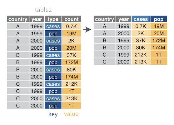
For example, table2 contains type, which is a column that repeats the variable names case and population. To make table2 tidy, you must move case and population values into their own columns.
## # A tibble: 12 x 4
##    country      year type            count
##    <chr>       <int> <chr>           <int>
##  1 Afghanistan  1999 cases             745
##  2 Afghanistan  1999 population   19987071
##  3 Afghanistan  2000 cases            2666
##  4 Afghanistan  2000 population   20595360
##  5 Brazil       1999 cases           37737
##  6 Brazil       1999 population  172006362
##  7 Brazil       2000 cases           80488
##  8 Brazil       2000 population  174504898
##  9 China        1999 cases          212258
## 10 China        1999 population 1272915272
## 11 China        2000 cases          213766
## 12 China        2000 population 1280428583
Solution
## # A tibble: 6 x 4
##   country      year  cases population
##   <chr>       <int>  <int>      <int>
## 1 Afghanistan  1999    745   19987071
## 2 Afghanistan  2000   2666   20595360
## 3 Brazil       1999  37737  172006362
## 4 Brazil       2000  80488  174504898
## 5 China        1999 212258 1272915272
## 6 China        2000 213766 1280428583
Discussion
To use spread(), assign the column that contains variable names to key. Assign the column that contains the values that are associated with those names to value. spread() will:
- Make a copy of the original table
- Remove the
keyandvaluecolumns from the copy - Remove every duplicate row in the data set that remains
- Insert a new column for each unique variable name in the
keycolumn Fill the new columns with the values of the
valuecolumn in a way that preserves every relationship between values in the original data setSince this is easier to see than explain, you may want to study the diagram and result above.
Each new column created by spread() will inherit the data type of the value column. If you would to convert each new column to the most sensible data type given its final contents, add the argument convert = TRUE.
3.7 Gather a field of cells into a pair of columns
You want to convert wide data to long, reshape a two-by-two table, or move variable values out of the column names and into the cells. These are different ways of describing the same action.
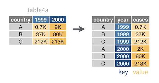
For example, table4a is a two-by-two table with the column names 1999 and 2000. These names are values of a year variable. The field of cells in table4a contains counts of TB cases, which is another variable. To make table4a tidy, you need to move year and case values into their own columns.
## # A tibble: 3 x 3
##   country     `1999` `2000`
## * <chr>        <int>  <int>
## 1 Afghanistan    745   2666
## 2 Brazil       37737  80488
## 3 China       212258 213766
Solution
## # A tibble: 6 x 3
##   country     year   cases
##   <chr>       <chr>  <int>
## 1 Afghanistan 1999     745
## 2 Brazil      1999   37737
## 3 China       1999  212258
## 4 Afghanistan 2000    2666
## 5 Brazil      2000   80488
## 6 China       2000  213766
Discussion
gather() is the inverse of spread(): gather() collapses a field of cells that spans several columns into two new columns:
- A column of former “keys”, which contains the column names of the former field
- A column of former “values”, which contains the cell values of the former field
To use gather(), pick names for the new key and value columns, and supply them as strings. Then identify the columns to gather into the new key and value columns. gather() will:
- Create a copy of the original table
- Remove the identified columns from the copy
- Add a key column with the supplied name
- Fill the key column with the column names of the removed columns, repeating rows as necessary so that each combination of row and removed column name appears once
- Add a value column with the supplied name
Fill the value column with the values of the removed columns in a way that preserves every relationship between values and column names in the original data set
Since this is easier to see than explain, you may want to study the diagram and result above.
Identify columns to gather
You can identify the columns to gather (i.e. remove) by:
- name
- index (numbers)
- inverse index (negative numbers that specifiy the columns to retain, all other columns will be removed.)
- the
select()helpers that come in the dplyr package
So for example, the following commands will do the same thing as the solution above:
table4a %>% gather(key = "year", value = "cases", `"1999", "2000")
table4a %>% gather(key = "year", value = "cases", -1)
table4a %>% gather(key = "year", value = "cases", one_of(c("1999", "2000")))
By default, the new key column will contain character strings. If you would like to convert the new key column to the most sensible data type given its final contents, add the argument convert = TRUE.
3.8 Separate a column into new columns
You want to split a single column into multiple columns by separating each cell in the column into a row of cells. Each new cell should contain a separate portion of the value in the original cell.
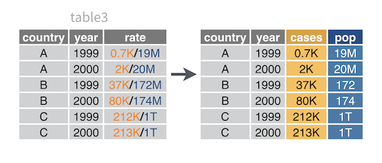
For example, table3 combines cases and population values in a single column named rate. To tidy table3, you need to separate rate into two columns: one for the cases variable and one for the population variable.
## # A tibble: 6 x 3
##   country      year rate
## * <chr>       <int> <chr>
## 1 Afghanistan  1999 745/19987071
## 2 Afghanistan  2000 2666/20595360
## 3 Brazil       1999 37737/172006362
## 4 Brazil       2000 80488/174504898
## 5 China        1999 212258/1272915272
## 6 China        2000 213766/1280428583
Solution
## # A tibble: 6 x 4
##   country      year  cases population
##   <chr>       <int>  <int>      <int>
## 1 Afghanistan  1999    745   19987071
## 2 Afghanistan  2000   2666   20595360
## 3 Brazil       1999  37737  172006362
## 4 Brazil       2000  80488  174504898
## 5 China        1999 212258 1272915272
## 6 China        2000 213766 1280428583
Discussion
To use separate(), pass col the name of the column to split, and pass into a vector of names for the new columns to split col into. You should supply one name for each new column that you expect to appear in the result; a mismatch will imply that something went wrong.
separate() will:
- Create a copy of the original data set
- Add a new column for each value of
into. The values will become the names of the new columns. - Split each cell of
colinto multiple values, based on the locations of a separator character. - Place the new values into the new columns in order, one value per column
Remove the
colcolumn. Add the argumentremove = FALSEto retain thecolcolumn in the final result.Since this is easier to see than explain, you may want to study the diagram and result above.
Each new column created by separate() will inherit the data type of the col column. If you would like to convert each new column to the most sensible data type given its final contents, add the argument convert = TRUE.
Control where cells are separated
By default, separate() will use non-alpha-numeric characters as a separators. Pass a regular expression to the sep argument to specify a different set of separators. Alternatively, pass an integer vector to the sep argument to split cells into sequences that each have a specific number of characters:
sep = 1will split each cell between the first and second character.sep = c(1, 3)will split each cell between the first and second character and then again between the third and fourth character.sep = -1will split each cell between the last and second to last character.
Separate into multiple rows
separate_rows() behaves like separate() except that it places each new value into a new row (instead of into a new column).
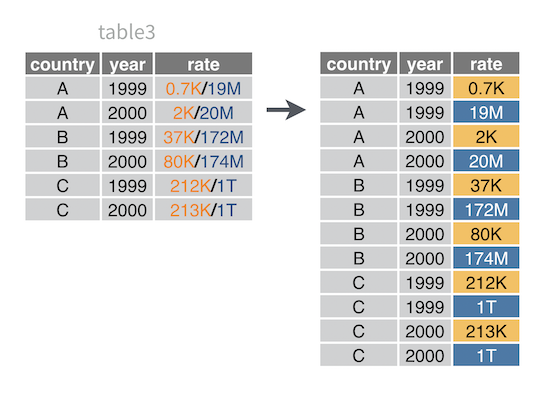
To use separate_rows(), follow the same syntax as separate().
3.9 Unite multiple columns into a single column
You want to combine several columns into a single column by uniting their values across rows.
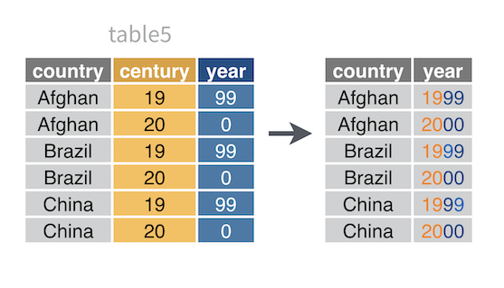
For example, table5 splits the year variable across two columns: century and year. To make table5 tidy, you need to unite century and year into a single column.
## # A tibble: 6 x 4
##   country     century year  rate
## * <chr>       <chr>   <chr> <chr>
## 1 Afghanistan 19      99    745/19987071
## 2 Afghanistan 20      00    2666/20595360
## 3 Brazil      19      99    37737/172006362
## 4 Brazil      20      00    80488/174504898
## 5 China       19      99    212258/1272915272
## 6 China       20      00    213766/1280428583
Solution
## # A tibble: 6 x 3
##   country     year  rate
##   <chr>       <chr> <chr>
## 1 Afghanistan 1999  745/19987071
## 2 Afghanistan 2000  2666/20595360
## 3 Brazil      1999  37737/172006362
## 4 Brazil      2000  80488/174504898
## 5 China       1999  212258/1272915272
## 6 China       2000  213766/1280428583
Discussion
To use unite(), give the col argument a character string to use as the name of the new column to create. Then list the columns to combine. Finally, give the sep argument a separator character to use to paste together the values in the cells of each column. unite() will:
- Create a copy of the original data set
- Paste together the values of the listed columns in a vectorized (i.e. rowwise) fashion.
unite()will place the value ofsepbetween each value during the paste process. - Append the results as a new column whose name is the value of
col Remove the listed columns. To retain the columns in the result, add the argument
remove = FALSE.Since this is easier to see than explain, you may want to study the diagram and result above.
sep value, unite() will use _ as a separator character. To avoid a separator character, use sep = "".